
本章目标:了解如何使用 Profiler 定位训练/推理中的性能瓶颈,包括 XLA/JAX profiler 和 NVIDIA 工具。
对应原书:Chapter 9 (How to Profile TPU Programs)
改写范围:原书主线是 JAX/XLA/XProf;Nsight、PyTorch Profiler 和常见 GPU 诊断流程是实践补充。 优先级:⭐ 低 | 建议时间:Day 13, 约 2 小时
13.1 为什么需要 Profiling
🔗 与你的联系
前面章节的 Roofline 分析都是”信封背面的估算”——假设硬件在理论极限运行。现实中,实际性能与理论之间有很大 gap。Profiling 就是用测量数据替代估算假设,找到真正拖慢系统的瓶颈。
理论 vs 现实的差距
| 假设 | 现实 |
|---|---|
| matmul 达到峰值 FLOPs | 受 layout/tiling 影响,MXU 利用率可能只有 50-80% |
| 通信与计算完美重叠 | 编译器不一定能做到 overlap |
| HBM 带宽持续满载 | 小 kernel 之间有 launch 开销,带宽利用不连续 |
| 内存分配无碎片 | 碎片化导致实际可用 HBM < 标称值 |
实际性能低于理论的常见原因:
- 编译器优化不足:生成的 kernel 没有达到理论最优(fusion 不充分)
- 内存布局问题:数据在 HBM 中的排列导致额外的 reshape/transpose/copy
- 流水线气泡:计算和通信没有完美重叠,GPU 有 idle 时间
- Kernel launch 开销:大量小 kernel 的 CPU→GPU 调度开销累积
- 内存碎片:HBM 利用不充分,峰值内存 > 实际活跃数据
Profiling 的价值
Profiling = 用数据说话。没有 profiler,优化就是猜测。
优化工作流:
1. Roofline 估算理论上界 → "应该能达到 X ms"
2. Profiler 测量实际时间 → "实际是 2X ms"
3. 分析 gap 来源 → "45% 时间花在 AllReduce 上"
4. 针对性优化 → 增加 gradient accumulation
5. 重新 profile → 验证效果
📋 背景知识:MFU(Model FLOPs Utilization)
MFU 是最常用的高级性能指标:
\[\text{MFU} = \frac{\text{实际有效 FLOPs/s}}{\text{硬件峰值 FLOPs/s}}\]
“有效 FLOPs” 指模型的理论 FLOPs($6NP$ per token),不包括 recompute 等冗余计算。
MFU 范围 含义 < 30% 严重问题(通常是通信或 data loading 瓶颈) 30-40% 有通信开销,但基本正常 40-50% 良好,典型的大规模训练 > 50% 优秀(需要高效 overlap + 良好的 batch size)
13.2 TPU/JAX 软件栈
编译流水线
JAX Python 代码(jnp.einsum, jnp.matmul 等)
    ↓ jax.jit / pjit(tracing)
StableHLO(平台无关的中间表示)
    ↓ XLA 前端
HLO(High Level Optimizer IR)
    ↓ XLA 优化 passes(fusion、layout、sharding)
LLO(Low Level Optimizer IR)
    ↓ 硬件特定代码生成
TPU 机器码 / CUDA PTX
📋 背景知识:编译器 IR(中间表示)
IR 是编译器内部的代码表示形式。就像 C 代码 → 汇编 → 机器码一样,JAX 也经过多层”翻译”:
- StableHLO:描述”做什么”(矩阵乘、加法等),不关心硬件
- HLO:加入了 fusion、layout 等优化决策
- LLO:直接对应硬件操作(systolic array 调度、DMA 传输等)
你在 profiler 中看到的是 HLO 层面的信息——它是理解性能的关键窗口。
XLA 编译器优化
XLA 是 Google 的加速线性代数编译器,负责将 HLO 转化为高效硬件指令。核心优化包括:
- Operator Fusion:将多个小操作合并成一个 kernel,避免中间结果写回 HBM
# 未 fusion: 3 次 HBM 读写 tmp1 = matmul(x, w) # 写回 HBM tmp2 = relu(tmp1) # 读+写 HBM out = dropout(tmp2) # 读+写 HBM # Fusion 后: 1 次读写 out = fused_matmul_relu_dropout(x, w) # 中间结果留在 VMEM/寄存器 -
Memory Layout Optimization:决定张量在 HBM 中的排列方式(行优先/列优先/tiling)
-
Communication Scheduling:安排 AllReduce 和 matmul 的重叠执行
- Sharding Propagation:根据用户指定的分片约束,自动推导中间张量的分片
HLO 语法入门
理解 HLO 对 profiling 非常重要。以下是一个简单的 JAX 程序及其 HLO:
import jax, jax.numpy as jnp

def multiply(x, y):
    return jnp.einsum('bf,fd->db', x, y)

y = jax.jit(multiply)(jnp.ones((128, 256)), jnp.ones((256, 16), dtype=jnp.bfloat16))
对应的 HLO(可通过 jax.jit(f).lower(*args).compile().as_text() 获取):
ENTRY %main.5 (Arg_0.1: f32[128,256], Arg_1.2: bf16[256,16]) -> f32[16,128] {
  %Arg_1.2 = bf16[256,16]{1,0} parameter(1)
  %convert.3 = f32[256,16]{1,0} convert(bf16[256,16]{1,0} %Arg_1.2)
  %Arg_0.1 = f32[128,256]{1,0} parameter(0)
  ROOT %dot.4 = f32[16,128]{1,0} dot(
      f32[256,16]{1,0} %convert.3,
      f32[128,256]{1,0} %Arg_0.1),
      lhs_contracting_dims={0}, rhs_contracting_dims={1}
}
可以看到:dot.4 就是矩阵乘,输入两个 f32 矩阵,沿第 0 和第 1 维收缩。convert.3 是将 bf16 转为 f32。
13.3 如何读懂 XLA Op
Profiler 中看到的每个操作都是一个 HLO op。学会读懂它们是 profiling 的核心技能。
Op 格式解析
%fusion.3 = bf16[32,32,4096]{2,1,0:T(8,128)(2,1)S(1)} fusion(
    bf16[32,32,8192]{2,1,0:T(8,128)(2,1)S(1)} %fusion.32),
    kind=kCustom, calls=%all-reduce-scatter.3
拆解各部分:
| 字段 | 示例 | 含义 |
|---|---|---|
| Op 名称 | fusion.3 |
操作的唯一标识。fusion 表示包含 ≤1 个 matmul + 若干逐元素操作 |
| 输出形状 | bf16[32,32,4096] |
dtype + 每维大小 |
| Layout | {2,1,0:T(8,128)(2,1)} |
维度在内存中的排列顺序 + tiling |
| 内存位置 | S(1) |
S(0)=HBM, S(1)=VMEM, S(2)/S(3)=其他 |
| 输入 | %fusion.32 |
上游 op 的引用 |
| 类型 | kind=kCustom |
op 类型(kCustom 常见于通信操作) |
Tiling 详解
Tiling 决定了 N 维数组在线性内存中的物理布局。例如:
f32[3,5]{1,0:T(2,2)}
逻辑视图 (3×5):           物理内存布局 (padded to 4×6):
┌─────────────────┐       ┌───┬───┬───┐
│ 0,0  0,1  0,2   │       │0,0│0,1│0,2│0,3│ ← tile (0,0) 和 (0,1)
│ 1,0  1,1  1,2   │  →    │1,0│1,1│1,2│1,3│
│ 2,0  2,1  2,2   │       ├───┼───┼───┤
│ 0,3  0,4        │       │2,0│2,1│2,2│2,3│ ← tile (1,0) 和 (1,1)
│ 1,3  1,4        │       │pad│pad│pad│pad│
│ 2,3  2,4        │       └───┴───┴───┘
└─────────────────┘
{1,0}→ 先行后列(行优先)T(2,2)→ 每 2×2 为一个 tile,tile 内行优先- Padding:3→4, 5→6(向上取到 tile 的整数倍),内存浪费 ≈ 1.6×
多层 tiling 示例:bf16[32,32,8192]{2,1,0:T(8,128)(2,1)S(1)}
- 外层 tiling T(8,128):按 8×128 分块
- 内层 tiling (2,1):bf16 的对齐要求(保证每次加载 ≥ 4 字节)
💡 为什么 tiling 影响性能?
TPU 的 systolic array 需要以特定的 tile 大小加载数据。如果张量的 layout 与硬件期望不匹配,XLA 会插入 copy/retile 操作来转换布局,这些操作消耗时间和带宽。在 profiler 中看到大量
copyop 通常意味着 layout 问题。JAX 提供实验性的
AUTOlayout 功能:jax.jit(f, in_shardings=AUTO)让 XLA 自动选择最优输入 layout。
13.4 JAX Profiler
JAX profiler 集成在 TensorBoard 中,通过 jax.profiler.trace() 捕获运行时信息:
import jax

with jax.profiler.trace("/tmp/tensorboard"):
    key = jax.random.key(0)
    x = jax.random.normal(key, (1024, 1024))
    y = x @ x
    y.block_until_ready()

# 查看:tensorboard --logdir=/tmp/tensorboard
Trace Viewer
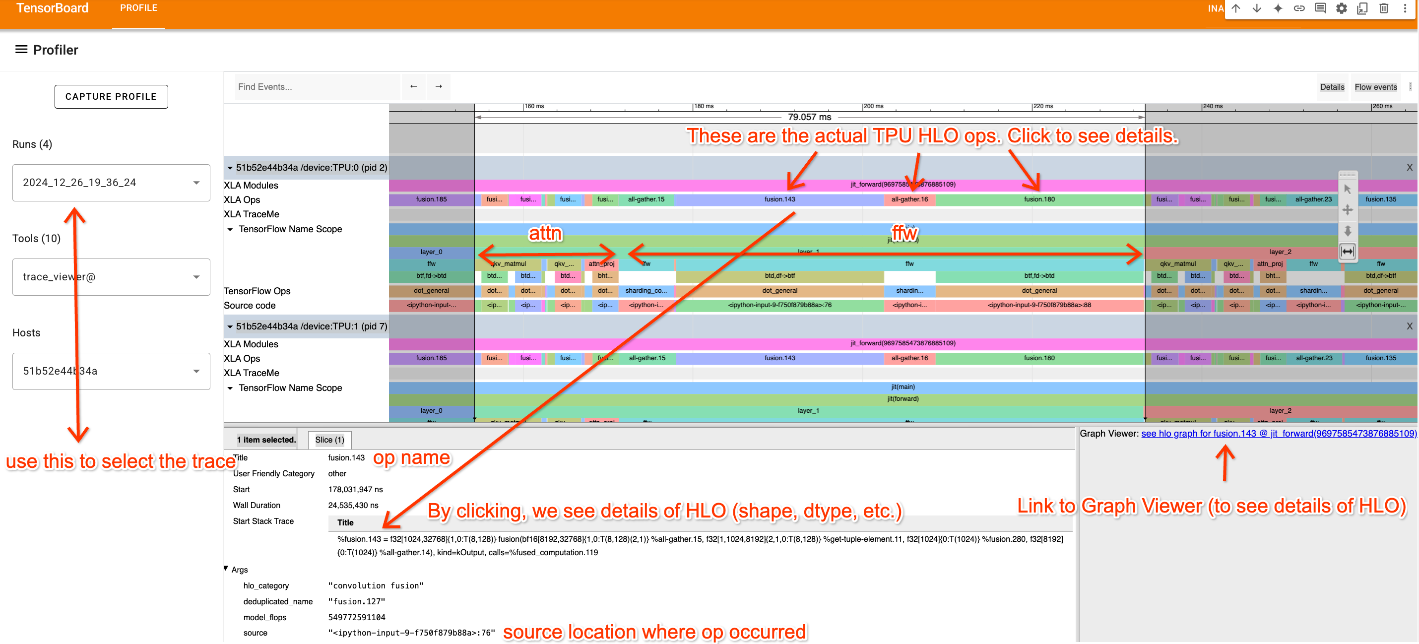
这是 profiler 中最有用的工具。 它展示每个 TPU/GPU 核心在时间轴上的所有动作:
- 顶层行(XLA Ops):实际的 TPU 操作(名称是 HLO op 名)
- 下方行:由
jax.named_scope和 Python 调用栈提供的语义标注 - 通信操作:AllReduce、ReduceScatter 等显示为独立的 fusion op
导航技巧:使用”游戏风格”控制——A/D 左右平移,W/S 缩放。点击任何 op 可查看:
- 来源代码行号
- HLO 完整文本
- 跳转到 Graph Viewer 的链接
如何识别 Transformer 各部分:
一个 Transformer 层的 Trace 示意:
┌──────────┬──────────┬──────┬──────────┬──────────┬──────┐
│  Q proj  │  K proj  │  V  │ Attention│  O proj  │ Comm │
│ (matmul) │ (matmul) │proj │  (dot)   │ (matmul) │(AR)  │
├──────────┴──────────┴──────┴──────────┴──────────┴──────┤
│                     Attention Block                      │
├──────────┬──────────┬──────┐                             │
│ Up proj  │Gate proj │ Down │                             │
│ (matmul) │(matmul)  │proj  │                             │
├──────────┴──────────┴──────┤                             │
│         MLP Block          │                             │
└────────────────────────────┘
XProf Overview
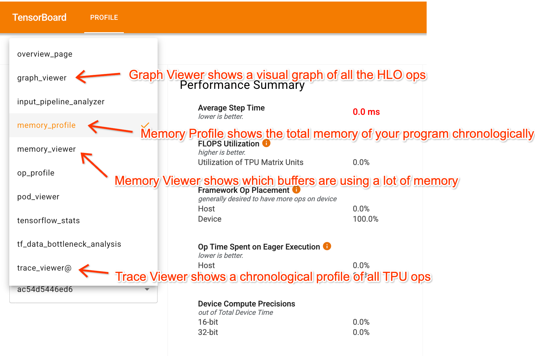
高级概览页面,一眼看到:
- 总步骤时间(step time)
- 各类操作的时间占比:matmul vs 通信 vs 逐元素 vs infeed/outfeed
- MXU 利用率:最重要的单一指标
Graph Viewer
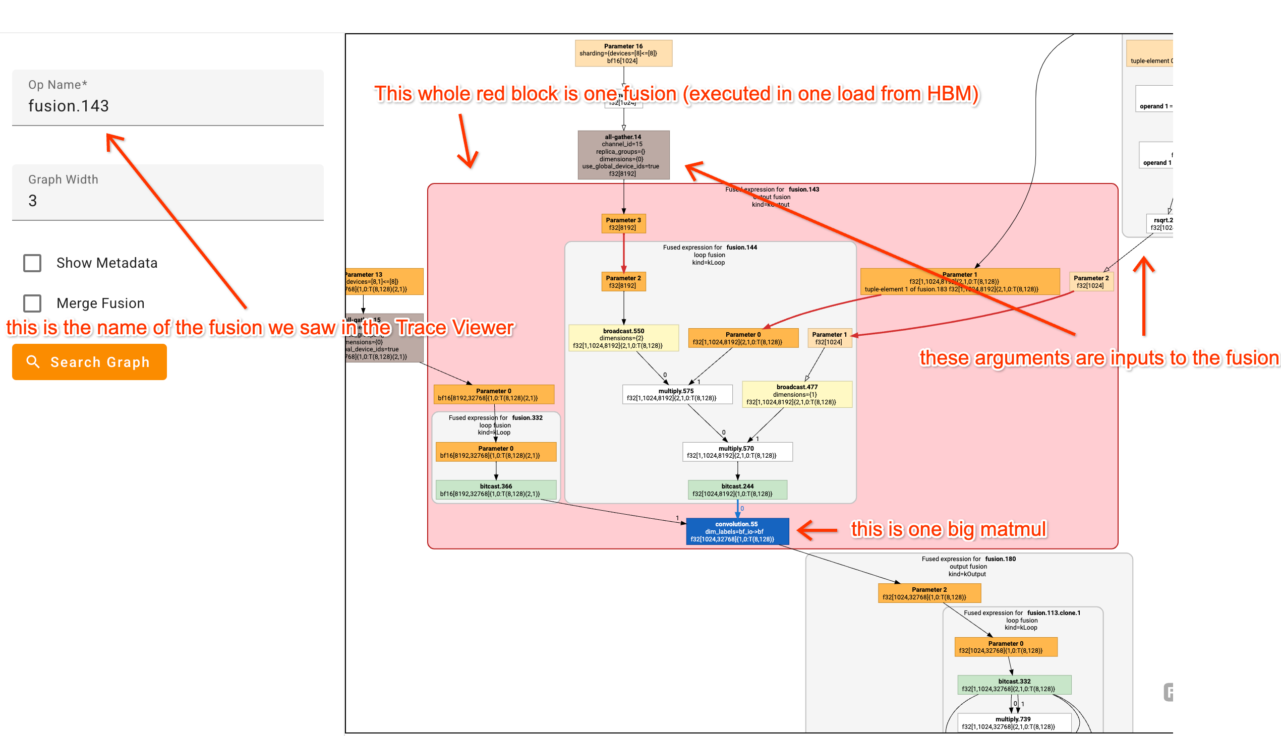
可视化 XLA 编译后的计算图。比直接读 HLO 文本容易很多:
- 每个节点是一个 XLA op,悬停可看到源代码位置
- 边是数据依赖(可以追踪某个 matmul 的输入来自哪里)
- 检查编译器是否做了预期的 fusion
- 查看分片决策:shape 中的维度变化反映了 sharding
Memory Profile
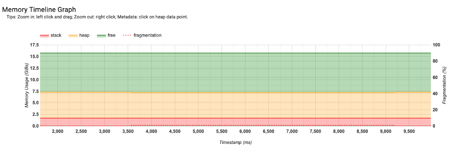
展示 HBM 使用随时间的变化:
- 峰值内存:是否接近 OOM 边界
- 参数内存(平坦的基线)vs 激活内存(训练时随 forward 增长,backward 后释放)
- KV cache(推理时随序列增长)
- 内存碎片:峰值 » 实际使用量可能意味着碎片化
13.5 实战:分析 Transformer 训练 Profile
FFW 块分析示例
假设我们在 8 片 TPU v2 上训练一个 Transformer(4-way DP, 2-way TP),profiler 显示 FFW 的 up-projection op:
输入: bf16[8, 1024, 8192] × bf16[8192, 16384]
输出: bf16[8, 1024, 16384]
耗时: 96 ms
验证是否达到 Roofline:
- 确定全局 shape:4-way DP → batch 维乘 4 = 32;2-way TP → hidden 维乘 2 = 32768
- 全局 matmul:
bf16[32, 1024, 8192] × bf16[8192, 32768]
- 全局 matmul:
-
计算 FLOPs:$2 \times 32 \times 1024 \times 8192 \times 32768 = 1.76 \times 10^{13}$
-
理论时间:$\frac{1.76 \times 10^{13}}{2.3 \times 10^{13} \times 8} = 95.6$ ms
- 实际 96 ms ≈ 理论值 → MXU 利用率接近 100%!
通信分析示例
FFW 末尾的 ReduceScatter op:
%fusion.1 = bf16[8,1024,4096]{2,1,0:T(8,128)(2,1)} fusion(
    bf16[8,1024,8192]{...} %fusion.31),
    kind=kCustom, calls=%all-reduce-scatter.1
分析:
- 输入 shape
bf16[8,1024,8192],每 shard = $2 \times 8 \times 1024 \times 8192 = 128$ MB - TPU v2 ICI 带宽 = $1.2 \times 10^{11}$ B/s(双向)
- 理论时间 = 128 MB / 120 GB/s ≈ 1.07 ms
- 实际 1.13 ms → 接近 Roofline!
Attention 块分析
Q projection 的 weight shape:[d_model=8192, n_heads=32, d_qkv=256]
使用 Megatron sharding 沿 head 维分片(2-way TP):
- 每 shard:
[8192, 16, 256]→ FLOPs = $2 \times 8 \times 1024 \times 8192 \times 4096 = 5.5 \times 10^{11}$ - 理论时间 ≈ 3 ms(compute-bound,因为 batch 足够大)
💡 Profile 分析的核心方法论
对每个 op:
- 从 HLO 读出 shape 和 dtype
- 结合分片信息推导全局 shape
- 计算理论 FLOPs / 加载字节数 / 通信量
- 对比 Roofline 预期时间
- 如果实际 » 理论:说明有优化空间(layout 问题?fusion 不充分?通信重叠不足?)
常见 Profile 问题模式
| Profile 中观察到的 | 含义 | 优化方向 |
|---|---|---|
大量 copy op |
Layout 不匹配,需要 retile | 使用 jax.jit(f, in_shardings=AUTO) |
| matmul 之间有 gap | 计算-通信未重叠 | 检查 XLA 的 overlap scheduling |
| AllReduce 时间 » 理论值 | 网络拥塞或路由不佳 | 检查拓扑和 ICI 带宽 |
| fusion 内多个小 op | VPU 操作聚合 | 正常现象,检查是否影响 MXU |
| Memory 峰值接近 OOM | 可能需要 checkpointing | 启用 gradient checkpointing |
13.6 NVIDIA GPU Profiling 工具
对于使用 Megatron/PyTorch + GPU 的场景,NVIDIA 提供了完整的工具链:
📋 背景知识:GPU Profiling 工具层次
高层(应用级)
  PyTorch Profiler / DeepSpeed Flops Profiler
    ↓ 输出 trace(JSON/Chrome Trace 格式)
中层(系统级)
  NVIDIA Nsight Systems (nsys)
    ↓ CUDA API calls、kernel 时间线、NCCL 通信
底层(kernel 级)
  NVIDIA Nsight Compute (ncu)
    ↓ 单 kernel 的 Roofline、SM 占用率、内存带宽
先 nsys 找瓶颈,再 ncu 深入分析是标准工作流。
NVIDIA Nsight Systems(nsys)
# 基础 profiling
nsys profile --trace=cuda,nvtx -o my_trace python train.py

# 限定范围(避免 profile 太大)
nsys profile --trace=cuda,nvtx \
  --capture-range=cudaProfilerApi \  # 只在代码标记的范围内采集
  --stats=true \                     # 输出统计摘要
  -o my_trace python train.py
输出 .nsys-rep 文件,在 Nsight Systems GUI 中打开。关键视图:
| 视图 | 对应 JAX Profiler | 用途 |
|---|---|---|
| CUDA Kernels 时间线 | Trace Viewer | 看 kernel 执行顺序和时长 |
| NCCL 通道 | 通信 op | 看 AllReduce/ReduceScatter 时间 |
| CPU Threads | — | 看 Python/CPU 开销(数据预处理) |
| GPU Context | — | 看 GPU 空闲时间(气泡) |
在 nsys 中识别 Megatron 的并行通信:
时间轴示意(nsys 输出):
GPU 0: ──[forward matmul]──[NCCL AllReduce]──[forward matmul]──
GPU 1: ──[forward matmul]──[NCCL AllReduce]──[forward matmul]──
GPU 2: ──[forward matmul]──[NCCL AllReduce]──[forward matmul]──
                            ↑
                     TP 通信(应该 overlap)
如果 AllReduce 和 matmul 之间有 gap → 通信未与计算重叠,需要检查 Megatron 的 --overlap-grad-reduce 选项。
NVIDIA Nsight Compute(ncu)
# 分析单个 kernel(选择最大的 matmul kernel)
ncu --set full \
  --kernel-name "volta_fp16_s884gemm" \  # 指定 kernel 名
  --launch-skip 100 --launch-count 5 \   # 跳过 warmup,只采集 5 次
  python train.py
ncu 提供 单 kernel 的 Roofline 分析:
Roofline Analysis:
  Achieved FLOPs: 312 TFLOPs/s (79% of peak)  ← 优秀
  Achieved HBM BW: 1.8 TB/s (90% of peak)     ← 接近 Roofline
  Compute vs Memory: Compute-bound             ← 符合预期

  SM Occupancy: 85%                            ← 足够高
  L2 Hit Rate: 45%                             ← 正常
ncu 的 Roofline 图会自动将你的 kernel 画在 Roofline 图上,让你一眼看出距离理论极限有多远。
PyTorch Profiler
import torch
from torch.profiler import profile, ProfilerActivity, schedule, tensorboard_trace_handler

with profile(
    activities=[ProfilerActivity.CPU, ProfilerActivity.CUDA],
    schedule=schedule(wait=1, warmup=1, active=3, repeat=2),
    on_trace_ready=tensorboard_trace_handler('./log_dir'),
    record_shapes=True,       # 记录张量 shape
    profile_memory=True,      # 记录内存分配
    with_stack=True,           # 记录 Python 调用栈
) as prof:
    for step, batch in enumerate(dataloader):
        train_step(batch)
        prof.step()
        if step >= 10:
            break
在 TensorBoard 中查看(tensorboard --logdir=./log_dir),可以看到:
- Kernel 时间线:每个 CUDA kernel 的执行时间
- Operator 视图:按 PyTorch operator 聚合(nn.Linear、F.gelu 等)
- Memory 时间线:GPU 内存分配/释放随时间的变化
- 调用栈:从 kernel 反查到 Python 代码行
torch.cuda.Event 手动计时
对于快速诊断,可以用 CUDA event 做精确计时:
start = torch.cuda.Event(enable_timing=True)
end = torch.cuda.Event(enable_timing=True)

start.record()
output = model(input)
end.record()
torch.cuda.synchronize()

print(f"Forward pass: {start.elapsed_time(end):.1f} ms")
🛠️ 实践:Megatron-LM Profiling
内置 Timer 系统
Megatron 在每个训练步骤自动输出时间分解:
[训练日志示例] iteration 100 | elapsed time per iteration (ms): 1234.5 | forward-compute: 456.2 | backward-compute: 567.3 | backward-params-all-reduce: 123.4 | optimizer: 87.6 | batch-generator: 0.0解读方法:
forward-compute+backward-compute应占总时间 > 70%backward-params-all-reduce对应 DP AllReduce → 如果占比 > 20%,考虑增加 gradient accumulation- 开启
--timing-log-level 2获取更细粒度的分解启用 nsys Profiling
# 在 Megatron 训练中启用 nsys
nsys profile --trace=cuda,nvtx \
  --capture-range=cudaProfilerApi \
  -o megatron_trace \
  python pretrain_gpt.py \
    --tensor-model-parallel-size 8 \
    --pipeline-model-parallel-size 4 \
    --profile \                    # Megatron 内置 flag
    --profile-step-start 10 \     # 从第 10 步开始
    --profile-step-end 15         # 到第 15 步结束
在 nsys 中查看 Megatron 的关键模式:
- TP AllReduce 是否与下一个 matmul 重叠
- PP 的 send/recv 是否有气泡(idle 时间)
- FSDP 的 AllGather 是否与计算重叠
Wandb 集成
--wandb-project my-project --wandb-exp-name my-experiment实时监控 MFU、吞吐量、loss、学习率。MFU 是最重要的高级指标。
NCCL 调试
export NCCL_DEBUG=INFO           # 打印通信初始化细节
export NCCL_DEBUG_SUBSYS=INIT    # 只看初始化(减少输出量)
export NCCL_P2P_DISABLE=0       # 确保 P2P 启用
export NCCL_IB_DISABLE=0        # 确保 IB 启用
MFU 瓶颈排查决策树
MFU < 30%?
├─ 是 → TP 跨节点?
│       ├─ 是 → 把 TP 限制在节点内
│       └─ 否 → 检查 data loading(batch-generator 时间)
├─ 30-40% → PP bubble 大?
│       ├─ 是 → 增加 micro-batch 数或用 interleaved PP
│       └─ 否 → 检查 AllReduce 时间(通信带宽不足?)
├─ 40-50% → 正常范围
│       └─ 尝试 --overlap-grad-reduce, --overlap-param-gather
└─ > 50% → 优秀
🛠️ 实践:SGLang / Mini-SGLang Profiling
Metrics Endpoint
curl http://localhost:30000/get_server_info | python -m json.tool关键指标:
指标 含义 预期值 cache_hit_rate前缀 KV cache 命中率 > 50%(有共享 prompt) num_running_reqs当前 decode batch size 接近 --max-running-requeststoken_usageKV cache 使用率 70-90%(太低浪费内存) avg_prefill_latency平均 TTFT 参考 12.3 节公式 avg_decode_latency平均 TPOT 参考 12.3 节公式 Benchmark 工具
python -m sglang.bench_serving \
  --backend sglang \
  --port 30000 \
  --dataset-name random \
  --num-prompts 1000 \
  --request-rate 10       # 10 QPS
输出包括 TTFT P50/P99、TPOT P50/P99、总吞吐量。对照第 12 章的理论值验证。
Mini-SGLang 的简化 Profiling
Mini-SGLang(
/Users/huabin/mini-sglang-main/)可以通过 Python 的 cProfile 分析调度开销:import cProfile cProfile.run('engine.step()', sort='cumulative')重点关注
scheduler.py中的schedule_batch()耗时——如果调度本身成为瓶颈,说明 batch 管理逻辑需要优化。
13.7 常见性能问题和解决方案
训练场景
| 症状 | Profiler 中表现 | 可能原因 | 解决方案 |
|---|---|---|---|
| MFU 很低 (< 30%) | AllReduce 占比 > 40% | TP 跨节点 | 确保 TP ≤ 节点内 GPU 数 |
| Step time 波动大 | CPU thread 有长 gap | Data loading 瓶颈 | 增加 dataloader workers |
| 通信 » 计算 | NCCL kernel 时间长 | DP AllReduce 太慢 | 增加 gradient accumulation |
| PP bubble 大 | GPU idle 段 > 20% | Micro-batch 太少 | 增加 micro-batch 或用 interleaved PP |
| OOM | Memory 峰值 = HBM | 激活值太大 | 启用 gradient checkpointing |
| 某些 GPU 比其他慢 | Trace 中一个 GPU 落后 | 负载不均 / 热降频 | 检查硬件健康、均衡分片 |
推理场景
| 症状 | 指标表现 | 可能原因 | 解决方案 |
|---|---|---|---|
| Decode 延迟高 | TPOT » 理论值 | 未量化 / TP 不足 | 增大 TP 或使用 int8/fp8 |
| TTFT 高 | Prefill latency 大 | Prompt 太长 | 增大 chunked-prefill-size |
| 吞吐量低 | batch 远小于临界值 | KV cache 内存不足 | 增加 GPU 或用 GQA/KV 量化 |
| 延迟抖动大 | TPOT P99 » P50 | Prefill 抢占 decode | 减小 chunked-prefill-size |
| Cache hit 低 | cache_hit_rate < 30% | 请求无共享前缀 | 启用 --schedule-policy lpm |
| GPU 利用率低 | SM occupancy < 50% | Batch 太小 | 增加并发请求 |
端到端优化 Checklist
□ 确认 TP 在节点内(NVLink)
□ 确认 batch size 接近临界值(训练),或 max-running-requests 合理(推理)
□ 确认 data loading 不是瓶颈(batch-generator < 5% step time)
□ 确认 gradient accumulation 足够(DP AllReduce 被 amortize)
□ 确认 memory 使用在 80-90%(太低=浪费,太高=OOM 风险)
□ 确认通信-计算 overlap 已启用(--overlap-grad-reduce)
□ 确认量化精度选择合理(推理: int8/fp8, 训练: bf16/fp8)
13.8 Worked Problems
Q1:解读 Mystery Profile
以下是一个 8 芯片 TPU 上的 profile 片段(只有 Trace Viewer 信息):
Op 1: reduce.6          | 0.5 ms
Op 2: fusion.1          | 12.3 ms
      → bf16[4096]{0:T(1024)} = fusion(
          bf16[4096,8192]{1,0:T(8,128)} %param.1,
          bf16[8192]{0:T(1024)} %reduce.6)
Op 3: fusion.2          | 11.8 ms
      → bf16[8192]{0:T(1024)} = fusion(
          bf16[8192,4096]{1,0:T(8,128)} %param.2,
          bf16[4096]{0:T(1024)} %fusion.1)
Op 4: all-reduce.1      | 2.1 ms
      → replica_groups={{0,16,32,48,64,80,96,112},...}
问题:这在做什么计算?全局 shape 是什么?分片方式是什么?
点击查看答案
分析:
- Op 2 和 Op 3 是两个矩阵乘:
- Op 2:
bf16[8192] × bf16[4096,8192] → bf16[4096](沿 8192 维收缩) - Op 3:
bf16[4096] × bf16[8192,4096] → bf16[8192](沿 4096 维收缩)
- Op 2:
-
all-reduce 的
replica_groups包含 8 个 replica(0,16,32,…)→ 8-way 模型并行 - 重构全局 shape:
- 每 shard 的 hidden dim × 8 → 全局 D = 8192×? 或 4096×?
- 输入
bf16[8192]是 batch dim(sharded per-device),全局 batch = 8192 - 权重
bf16[4096,8192]中 4096 = D_ff / 8 → 全局 D_ff = 32768 - 全局:
[8, 8192] × [32768, 8192] → [8, 32768],然后[8, 32768] × [8192, 32768] → [8, 8192]
- 这是一个 MLP 块的 forward pass! up-projection + down-projection,8-way TP 沿 D_ff 维分片。
Q2:验证 Roofline 与修复 Sharding
一个简单 Transformer 在 8 片 TPU v2 上的 profile 显示每层 184 ms,但理论应该只有 ~90 ms。
问题:可能的原因是什么?如何修复?
点击查看答案
184 ms vs 90 ms → 效率只有 49%。 可能原因:
-
Sharding 不正确:XLA 的 GSPMD 分片传播可能做出了次优决策。例如,MLP 的权重沿错误维度分片 → matmul 变成了在通信维度上的 reduce。
-
Layout 问题:tensor 的物理 layout 与 matmul 要求不匹配 → 插入了大量 copy/retile 操作。
修复方法:使用 jax.lax.with_sharding_constraint 显式约束中间张量的分片:
from jax.sharding import PartitionSpec as P

def transformer_layer(x, w_up, w_down):
    # 显式约束 x 的分片
    x = jax.lax.with_sharding_constraint(x, P('data', None))

    # MLP up projection
    h = jnp.einsum('bd,df->bf', x, w_up)
    h = jax.lax.with_sharding_constraint(h, P('data', 'model'))

    # MLP down projection
    y = jnp.einsum('bf,fd->bd', h, w_down)
    y = jax.lax.with_sharding_constraint(y, P('data', None))
    return y
修复后通常能从 184 ms 降到 ~67 ms(原书数据)。
Q3:GPU 训练 MFU 诊断
你的 Megatron-LM 训练在 64 张 H100 上报告 MFU = 28%。配置:TP=8, PP=2, DP=4, LLaMA 70B。
问题:如何系统地诊断和优化?
点击查看答案
步骤 1:检查时间分解(Megatron 内置 timer)
forward-compute: 350 ms
backward-compute: 700 ms
backward-params-all-reduce: 450 ms  ← 占 36%!异常高
optimizer: 100 ms
batch-generator: 5 ms
total: 1605 ms
AllReduce 占 36% → DP 通信是瓶颈。
步骤 2:计算理论 AllReduce 时间
DP=4, 模型 70B×2 bytes = 140 GB。Ring AllReduce 理论时间:
\[T_{AR} = \frac{2(N-1)}{N} \times \frac{\text{size}}{\text{bandwidth}} = \frac{6}{4} \times \frac{140 \times 10^9}{4 \times 10^{11}} = 525 \text{ ms (IB)}\]但实际应该被 gradient accumulation 分摊!如果 gradient accumulation = 1 → 每步都做全量 AllReduce。
步骤 3:解决方案
- 增加 gradient accumulation steps = 4 → AllReduce 分摊到 4 步 → 有效通信时间 112 ms
- 或启用
--overlap-grad-reduce:与 backward 计算重叠 - 或增大 DP(减小 per-device batch),减少每次 AllReduce 的数据量
步骤 4:验证 PP bubble
PP=2, micro-batch=8: bubble = (PP-1)/(M+PP-1) = 1/9 ≈ 11%。这是合理的。
预期优化后 MFU:28% × (1605 / (1605-450+112)) = 28% × 1.27 ≈ 35%。进一步加 overlap 可到 40%+。
Q4:推理延迟异常诊断
SGLang 部署 LLaMA 70B(TP=8, 8×H100),理论 TPOT ≈ 5.2 ms,但实测 P50 = 12 ms, P99 = 45 ms。
问题:可能的原因和诊断方法?
点击查看答案
P50 = 12 ms(理论的 2.3×):
- 检查 batch size:如果
num_running_reqs≈ 200,KV cache 加载时间 ≈ 6 ms → 总 11 ms,接近观测值 - 结论:batch 太大导致 KV 加载主导。减小
--max-running-requests或启用 KV cache 量化
P99 = 45 ms(4× P50):
- Prefill 抢占:长 prompt 的 prefill 与 decode 竞争 GPU
- 减小
--chunked-prefill-size(如 2048→1024),让 prefill 更频繁地让出 GPU
诊断工具:
# 用 nsys 捕获推理
nsys profile --trace=cuda,nvtx \
  --capture-range=cudaProfilerApi \
  -o sglang_trace \
  python -m sglang.launch_server ...
在 trace 中查看:decode step 之间是否有大的 prefill chunk 插入(应该看到交替的小 decode + 偶尔的大 prefill chunk)。
关键要点
| 概念 | 要点 |
|---|---|
| Profiling 目的 | 用数据定位真正瓶颈,避免盲目优化 |
| 编译流水线 | JAX → StableHLO → HLO → LLO → 机器码 |
| 读懂 HLO | 掌握 op 名称、shape、layout (tiling)、内存位置的含义 |
| Trace Viewer | 最有用的工具——看 kernel 时间线、识别 gap 和通信 |
| Roofline 验证 | 对每个 op 计算理论时间,对比实际时间 |
| GPU 工具链 | nsys(系统级)→ ncu(kernel 级)→ PyTorch Profiler(应用级) |
| Megatron 诊断 | 内置 timer + nsys + MFU 瓶颈决策树 |
| SGLang 诊断 | metrics endpoint + bench_serving + 对照理论公式 |
| MFU 分级 | < 30% 严重问题,30-40% 通信瓶颈,40-50% 正常,> 50% 优秀 |